---
title: "Conditional Probability and Bayes' Theorem"
subtitle: "Updating Beliefs with New Information"
author: "Universe Office"
date: 2026-04-04
categories: [probability, foundations]
bibliography: references.bib
format:
html:
code-fold: true
toc: true
---
## Introduction
A medical test for a rare disease comes back positive. The test is 99% accurate. Should you be worried? Most people's gut reaction is "yes, almost certainly." But the mathematics tells a different story: if the disease affects only 1 in 1,000 people, a positive result means you have roughly a 2% chance of actually being sick. The other 98% are false positives.
This counterintuitive result --- and the framework for reasoning about it correctly --- is what this article is about.
The [previous article](../expectation-variance/index.qmd) introduced expectation and variance --- summary measures that describe the center and spread of a distribution. Those measures assume you observe the random variable directly, with no additional context. In practice, you rarely start from zero. A test returns positive. A borrower misses a payment. A contestant picks a door. Each piece of information changes what you know, and your probability estimates should change with it.
**Conditional probability** formalizes this update [@casella2002]. **Bayes' theorem** turns it into a computational tool: given new evidence, how should you revise your beliefs? [@wasserman2004]
Think of conditional probability as a **spotlight**: it narrows the stage to only the outcomes consistent with what you have observed, then rescales the probabilities so they still sum to 1.
This article covers:
- Conditional probability and the multiplication rule
- Independence and conditional independence
- The law of total probability
- Bayes' theorem and posterior updating
- Practical simulations: the Monty Hall problem and naive Bayes intuition
## Conditional Probability
### Definition
::: {.callout-note}
## Definition (Conditional Probability; Casella & Berger, 2002)
For events $A$ and $B$ with $P(B) > 0$, the **conditional probability** of $A$ given $B$ is:
$$
P(A \mid B) = \frac{P(A \cap B)}{P(B)}
$$
:::
The definition says: restrict attention to the outcomes where $B$ occurred, then ask how often $A$ also occurs within that restricted space. The denominator $P(B)$ renormalizes so that the conditional probabilities sum to 1.
### Multiplication Rule
Rearranging the definition gives the **multiplication rule**:
$$
P(A \cap B) = P(A \mid B) \cdot P(B) = P(B \mid A) \cdot P(A)
$$
This extends to chains of events:
$$
P(A_1 \cap A_2 \cap \cdots \cap A_n) = P(A_1) \cdot P(A_2 \mid A_1) \cdot P(A_3 \mid A_1 \cap A_2) \cdots P(A_n \mid A_1 \cap \cdots \cap A_{n-1})
$$
### Example: Dice and Cards
```{python}
#| label: conditional-basic
# Fair die: P(even | >= 3)
# Sample space restricted to {3,4,5,6}, even outcomes = {4,6}
p_even_given_ge3 = 2 / 4
print(f"P(even | die >= 3) = {p_even_given_ge3:.4f}")

# Standard deck: P(King | Face card)
# Face cards = 12 (J, Q, K in 4 suits), Kings = 4
p_king_given_face = 4 / 12
print(f"P(King | face card) = {p_king_given_face:.4f}")

# Verify via definition: P(King AND face) / P(face)
p_king_and_face = 4 / 52  # All kings are face cards
p_face = 12 / 52
print(f"Verification: {p_king_and_face / p_face:.4f}")
```
@fig-conditional shows a Venn diagram illustrating conditional probability. The shaded region represents $A \cap B$ relative to $B$.
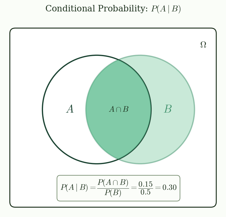{#fig-conditional}
## Independence
### Definition
::: {.callout-note}
## Definition (Independence; Casella & Berger, 2002)
Events $A$ and $B$ are **independent** if:
$$
P(A \cap B) = P(A) \cdot P(B)
$$
Equivalently, $P(A \mid B) = P(A)$ --- knowing $B$ occurred tells you nothing about $A$.
:::
### Pairwise vs. Mutual Independence
This distinction is subtle but important. Three events $A$, $B$, $C$ are **pairwise independent** if each pair is independent:
$$
P(A \cap B) = P(A)P(B), \quad P(A \cap C) = P(A)P(C), \quad P(B \cap C) = P(B)P(C)
$$
They are **mutually independent** if, in addition:
$$
P(A \cap B \cap C) = P(A) \cdot P(B) \cdot P(C)
$$
**Pairwise independence does not imply mutual independence.** Here is a concrete example: flip two fair coins. Define:
- $A$ = "first coin is heads"
- $B$ = "second coin is heads"
- $C$ = "exactly one head"
Check pairwise: $P(A) = P(B) = P(C) = 1/2$. For each pair, $P(A \cap B) = 1/4 = P(A)P(B)$, and similarly for the other pairs. But $P(A \cap B \cap C) = 0$ (you cannot have both coins heads *and* exactly one head), while $P(A)P(B)P(C) = 1/8$. The three events are pairwise independent but not mutually independent.
### Conditional Independence
Events $A$ and $B$ are **conditionally independent** given $C$ if:
$$
P(A \cap B \mid C) = P(A \mid C) \cdot P(B \mid C)
$$
Conditional independence does not imply marginal independence, and vice versa. This distinction matters in probabilistic graphical models and Bayesian networks.
### Simulation: Verifying Independence
```{python}
#| label: independence-sim
import numpy as np

rng = np.random.default_rng(seed=12345)
n = 1_000_000

# Two independent fair dice
die1 = rng.integers(1, 7, size=n)
die2 = rng.integers(1, 7, size=n)

# A = "die1 is even", B = "die2 > 3"
a = die1 % 2 == 0
b = die2 > 3

p_a = a.mean()
p_b = b.mean()
p_ab = (a & b).mean()

print(f"P(A)         = {p_a:.4f}  (theory: 0.5000)")
print(f"P(B)         = {p_b:.4f}  (theory: 0.5000)")
print(f"P(A ∩ B)     = {p_ab:.4f}  (theory: 0.2500)")
print(f"P(A) × P(B)  = {p_a * p_b:.4f}")
print(f"Independent?   {abs(p_ab - p_a * p_b) < 0.005}")
```
## Law of Total Probability
### Partition
A **partition** of the sample space $\Omega$ is a collection of mutually exclusive, exhaustive events $\{B_1, B_2, \ldots, B_n\}$: the $B_i$ are disjoint and $\bigcup_i B_i = \Omega$.
### Theorem
::: {.callout-note}
## Law of Total Probability (Casella & Berger, 2002)
If $\{B_1, B_2, \ldots, B_n\}$ is a partition of $\Omega$ with $P(B_i) > 0$ for all $i$, then for any event $A$:
$$
P(A) = \sum_{i=1}^{n} P(A \mid B_i) \cdot P(B_i)
$$
:::
**Proof.** Since $\{B_i\}$ is a partition, $A = \bigcup_i (A \cap B_i)$ where the union is disjoint. By the third axiom of probability and the multiplication rule:
$$
P(A) = \sum_i P(A \cap B_i) = \sum_i P(A \mid B_i) \cdot P(B_i) \qquad \square
$$
### Example: Factory Defect Rate
A factory has two production lines. Line 1 produces 60% of output with a 2% defect rate; Line 2 produces 40% with a 5% defect rate. What is the overall defect rate?
```{python}
#| label: total-probability
# P(defect) via law of total probability
p_line1, p_line2 = 0.60, 0.40
p_defect_line1, p_defect_line2 = 0.02, 0.05

p_defect = p_defect_line1 * p_line1 + p_defect_line2 * p_line2
print(f"P(defect) = {p_defect_line1}×{p_line1} + {p_defect_line2}×{p_line2}")
print(f"          = {p_defect:.4f}")
```
## Bayes' Theorem
### The Key Insight: Inverting the Direction
Bayes' theorem answers the question you usually *actually* want to ask. You observe evidence and want to know which hypothesis is most likely. But what you typically *have* is the reverse: the probability of evidence under each hypothesis.
Bayes' theorem inverts that direction.
::: {.callout-note}
## Bayes' Theorem (Bayes, 1763; Casella & Berger, 2002)
$$
P(B_j \mid A) = \frac{P(A \mid B_j) \cdot P(B_j)}{\sum_{i=1}^{n} P(A \mid B_i) \cdot P(B_i)}
$$
:::
The ingredients have specific names:
- **Prior**: $P(B_j)$ --- your belief before observing evidence
- **Likelihood**: $P(A \mid B_j)$ --- how probable the evidence is under each hypothesis
- **Posterior**: $P(B_j \mid A)$ --- your updated belief after observing evidence
The relationship is simple: **posterior $\propto$ likelihood $\times$ prior**. New evidence does not replace your prior beliefs --- it *updates* them. Strong evidence shifts the posterior far from the prior. Weak evidence barely moves it.
### Example: Medical Test (Sensitivity and Specificity)
A disease affects 1 in 1,000 people. A test has 99% sensitivity (true positive rate) and 95% specificity (true negative rate). You test positive. What is the probability you have the disease?
```{python}
#| label: bayes-medical
prevalence = 0.001
sensitivity = 0.99   # P(positive | disease)
specificity = 0.95   # P(negative | no disease)
fpr = 1 - specificity  # false positive rate

# P(positive) via total probability
p_positive = sensitivity * prevalence + fpr * (1 - prevalence)

# Bayes' theorem: P(disease | positive)
p_disease_given_pos = (sensitivity * prevalence) / p_positive

print(f"Prevalence:         {prevalence}")
print(f"Sensitivity:        {sensitivity}")
print(f"Specificity:        {specificity}")
print(f"P(positive):        {p_positive:.6f}")
print(f"P(disease|positive): {p_disease_given_pos:.4f}")
print(f"\nDespite 99% sensitivity, a positive test means only "
      f"a {p_disease_given_pos:.1%} chance of disease.")
print("The low prevalence overwhelms the test's accuracy.")
```
@fig-bayes compares the prior and posterior probabilities. The false positive paradox becomes visually clear.
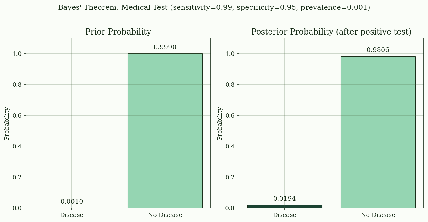{#fig-bayes}
### Effect of Prevalence
The posterior depends critically on prevalence. When the disease is rare, even a highly accurate test produces mostly false positives --- because the large number of healthy people tested generates more false alarms than the small number of sick people generates true alarms. @fig-medical-test shows how the positive predictive value changes as prevalence increases.
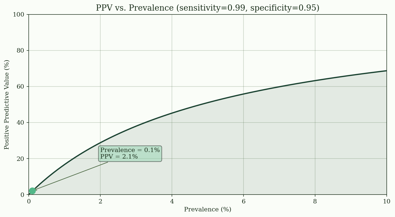{#fig-medical-test}
## Practical Examples
### The Monty Hall Problem
A game show has three doors: behind one is a car, behind the other two are goats. You pick a door. The host, who knows where the car is, opens another door to reveal a goat. Should you switch?
Bayes' theorem says **yes, always switch**. Switching wins with probability $2/3$; staying wins with probability $1/3$.
**Intuition via Bayes' theorem.** Suppose you pick Door 1.
- **Prior**: $P(\text{car at door } i) = 1/3$ for each $i$
- The host opens a goat door (say Door 3). This is certain if the car is at Door 2, but only happens half the time if the car is at Door 1.
- **Posterior**: $P(\text{car at door 2} \mid \text{host opens door 3}) = 2/3$
The key insight: your initial pick had a 1/3 chance of being right. That does not change when the host opens a door. The host's action concentrates the remaining 2/3 probability onto the one unopened door.
```{python}
#| label: monty-hall
import numpy as np

rng = np.random.default_rng(seed=12345)
n = 100_000

car = rng.integers(0, 3, size=n)
choice = rng.integers(0, 3, size=n)

# Staying wins when initial choice == car position
stay_wins = (choice == car).mean()
switch_wins = (choice != car).mean()

print(f"Simulated over {n:,} games:")
print(f"  Stay:   win rate = {stay_wins:.4f}  (theory: 1/3 ≈ 0.3333)")
print(f"  Switch: win rate = {switch_wins:.4f}  (theory: 2/3 ≈ 0.6667)")
```
@fig-monty-hall shows the simulation results converging to the theoretical values.
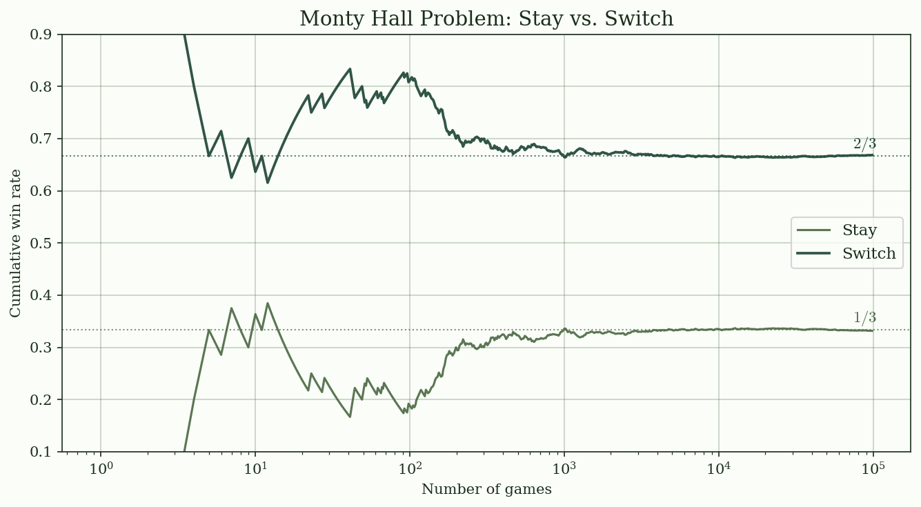{#fig-monty-hall}
### Spam Filter: Naive Bayes Intuition
Bayesian reasoning powers one of the simplest and most effective text classifiers. Given a message with word $w$, a naive Bayes classifier computes:
$$
P(\text{spam} \mid w) = \frac{P(w \mid \text{spam}) \cdot P(\text{spam})}{P(w \mid \text{spam}) \cdot P(\text{spam}) + P(w \mid \text{ham}) \cdot P(\text{ham})}
$$
The "naive" assumption is that words are conditionally independent given the class. This is clearly wrong linguistically, but works surprisingly well in practice.
```{python}
#| label: naive-bayes
# Toy example: word "free" in spam vs. ham
p_spam = 0.3
p_ham = 0.7
p_free_given_spam = 0.80
p_free_given_ham = 0.05

# P(spam | "free")
p_free = p_free_given_spam * p_spam + p_free_given_ham * p_ham
p_spam_given_free = (p_free_given_spam * p_spam) / p_free

print(f"P(spam)             = {p_spam}")
print(f"P('free' | spam)    = {p_free_given_spam}")
print(f"P('free' | ham)     = {p_free_given_ham}")
print(f"P(spam | 'free')    = {p_spam_given_free:.4f}")
print(f"\nSeeing 'free' raises spam probability from "
      f"{p_spam:.0%} to {p_spam_given_free:.1%}.")
```
## Summary and Connections
This article introduced conditional probability and Bayes' theorem --- the tools for updating probabilities when new information arrives. Key takeaways:
- Conditional probability restricts the sample space to what is known and renormalizes
- The multiplication rule decomposes joint probabilities into conditional chains
- Independence means one event carries no information about another. Pairwise independence is strictly weaker than mutual independence --- the coin-flip example shows they are not the same.
- The law of total probability marginalizes over a partition
- Bayes' theorem inverts conditioning: from $P(\text{evidence} \mid \text{hypothesis})$ to $P(\text{hypothesis} \mid \text{evidence})$
- Even highly accurate tests produce many false positives when the base rate is low
**Next**: [The Law of Large Numbers and Central Limit Theorem](../lln-clt/index.qmd) --- what happens when you average many random variables? Two foundational theorems describe the convergence behavior.
**Application preview**: Conditional probability is pervasive in credit risk. The probability of default conditional on macroeconomic stress ($PD \mid \text{downturn}$) underpins regulatory stress testing. In IFRS 9, the transition between ECL stages is a conditional probability problem: a loan moves from Stage 1 to Stage 2 when its credit risk has increased significantly since initial recognition, which is evaluated through conditional PD changes. Bayes' theorem also provides the framework for updating PD estimates as new borrower information arrives.
## References
::: {#refs}
:::


