---
title: "Random Variables"
subtitle: "From Sample Spaces to Measurable Functions"
author: "Universe Office"
date: 2026-04-04
categories: [probability, foundations]
bibliography: references.bib
format:
html:
code-fold: true
toc: true
---
## Introduction
Suppose you roll two dice and want to know the total. The sample space has 36 outcomes --- $(1,1), (1,2), \ldots, (6,6)$ --- but you do not care which specific pair appears. You only care about the sum. That sum is a function that converts each outcome into a number: $(1,3) \mapsto 4$, $(5,6) \mapsto 11$, and so on.
This is the idea behind a **random variable**: a rule that assigns a real number to every outcome in the sample space $\Omega$. Why not work with $\Omega$ directly? Because $\Omega$ can be anything --- coin labels, weather states, loan outcomes --- but arithmetic requires numbers. A random variable is the bridge from abstract outcomes to the concrete world of sums, averages, and integrals.
Think of a random variable as a **translator**: it listens to what the probability space says (in its native language of outcomes) and writes it down as a number you can compute with.
The [previous article](../probability-space/index.qmd) established the probability space $(\Omega, \mathcal{F}, P)$. This article introduces the tool that makes that foundation quantitatively useful [@casella2002; @wasserman2004].
This article covers:
- The formal definition of a random variable as a measurable function
- Discrete vs. continuous random variables
- PMF, PDF, and CDF
- Transformations of random variables
- Simulation and visual verification
## From Dice Sums to the Formal Definition
### Why We Need Random Variables
Consider the two-dice example. The sample space $\Omega = \{(i, j) : i, j \in \{1,\ldots,6\}\}$ has 36 elements. If you want the probability that the total is 7, you must count pairs: $(1,6), (2,5), (3,4), (4,3), (5,2), (6,1)$. The random variable $X(\omega) = i + j$ maps each pair to its sum, letting you write $P(X = 7) = 6/36 = 1/6$ without enumerating outcomes every time.
This pattern repeats everywhere. In credit risk, you do not track every borrower attribute --- you summarize default as $D = 1$ or $D = 0$. In physics, you measure a particle's position, not the full microstate of the system. Random variables extract the numerical quantity you care about from the richer probability space underneath.
### The Formal Definition
::: {.callout-note}
## Definition (Random Variable; Casella & Berger, 2002)
A **random variable** is a measurable function $X : \Omega \to \mathbb{R}$. "Measurable" means that for every Borel set $B \subseteq \mathbb{R}$, the preimage $X^{-1}(B) = \{\omega \in \Omega : X(\omega) \in B\}$ belongs to $\mathcal{F}$.
:::
In practice, the measurability condition ensures that you can always ask "what is the probability that $X$ falls in the interval $[a, b]$?" and get a well-defined answer. For finite or countable sample spaces, every function from $\Omega$ to $\mathbb{R}$ is automatically measurable. The condition only bites in continuous settings, where it rules out pathological functions that would break the probability machinery.
## Discrete vs. Continuous
A random variable $X$ is **discrete** if it takes values in a countable set $\{x_1, x_2, \ldots\}$. It is **continuous** if its CDF is absolutely continuous --- equivalently, if there exists a density function $f$ such that $P(a \le X \le b) = \int_a^b f(x)\,dx$ for all $a \le b$.
The intuition: a discrete random variable assigns probability to individual points (like landing on a specific face of a die). A continuous random variable spreads probability over intervals (like a spinner that can land anywhere on a circle).
```{python}
#| label: discrete-continuous-example
from scipy import stats

# Discrete: Binomial(n=20, p=0.3)
X_binom = stats.binom(n=20, p=0.3)
print(f"P(X = 6)  = {X_binom.pmf(6):.4f}")
print(f"P(X <= 6) = {X_binom.cdf(6):.4f}")

# Continuous: Normal(0, 1)
X_norm = stats.norm(0, 1)
print(f"f(0)      = {X_norm.pdf(0):.4f}")
print(f"P(X <= 0) = {X_norm.cdf(0):.4f}")
```
## Probability Mass Function and Probability Density Function
### PMF (Discrete): Probability Lives on Points
For a discrete random variable, you can ask "what is the probability of *exactly* this value?" The answer is the **probability mass function** (PMF):
$$
p(x) = P(X = x)
$$
The PMF satisfies $p(x) \ge 0$ for all $x$, and $\sum_x p(x) = 1$. Visually, a PMF is a **bar chart** --- each bar's height is the probability of that value.
### PDF (Continuous): Probability Lives in Areas
For a continuous random variable, the probability of any single point is zero. Instead, probability comes from *intervals*. The **probability density function** (PDF) satisfies:
$$
P(a \le X \le b) = \int_a^b f(x)\,dx
$$
Note that $f(x)$ is *not* a probability --- it can exceed 1. What must equal 1 is the total area under the curve: $\int_{-\infty}^{\infty} f(x)\,dx = 1$. Visually, a PDF is a **smooth curve**, and probability is the **area under the curve** between two points.
@fig-pmf-pdf shows six common distributions: three discrete (Bernoulli, Binomial, Poisson) and three continuous (Normal, Exponential, Uniform).
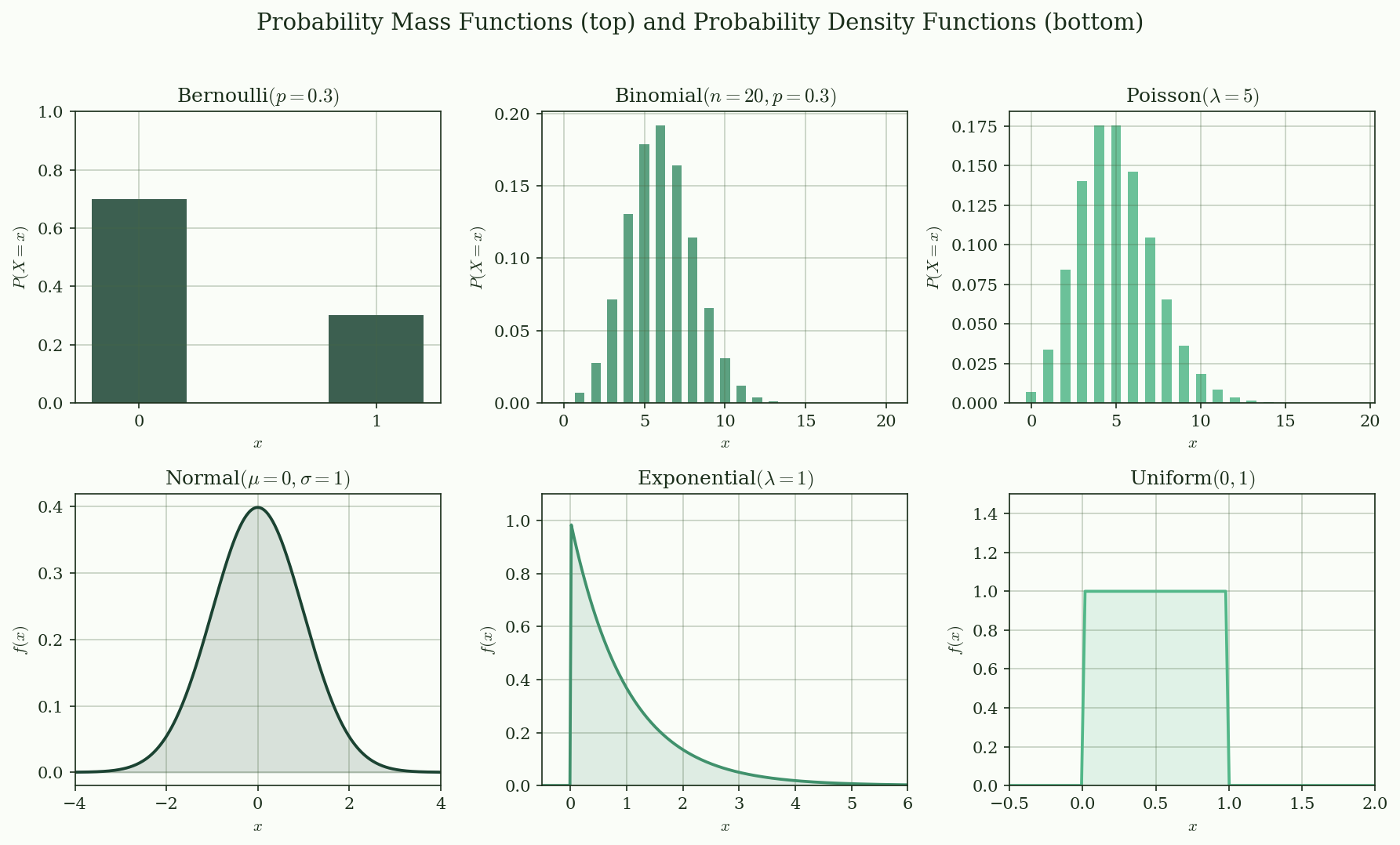{#fig-pmf-pdf}
## Cumulative Distribution Function
The **CDF** unifies discrete and continuous cases into a single framework:
$$
F(x) = P(X \le x)
$$
Every CDF has three properties (Casella & Berger, 2002):
1. **Non-decreasing**: $x_1 < x_2 \implies F(x_1) \le F(x_2)$
2. **Right-continuous**: $\lim_{h \to 0^+} F(x + h) = F(x)$
3. **Limits**: $\lim_{x \to -\infty} F(x) = 0$ and $\lim_{x \to \infty} F(x) = 1$
For discrete random variables, the CDF is a step function with jumps at each value. For continuous random variables, the PDF and CDF are related by:
$$
F(x) = \int_{-\infty}^{x} f(t)\,dt, \qquad f(x) = F'(x)
$$
@fig-cdf illustrates this relationship for $N(0, 1)$. The shaded area under the PDF up to $x = 1.0$ equals $F(1.0) \approx 0.841$.
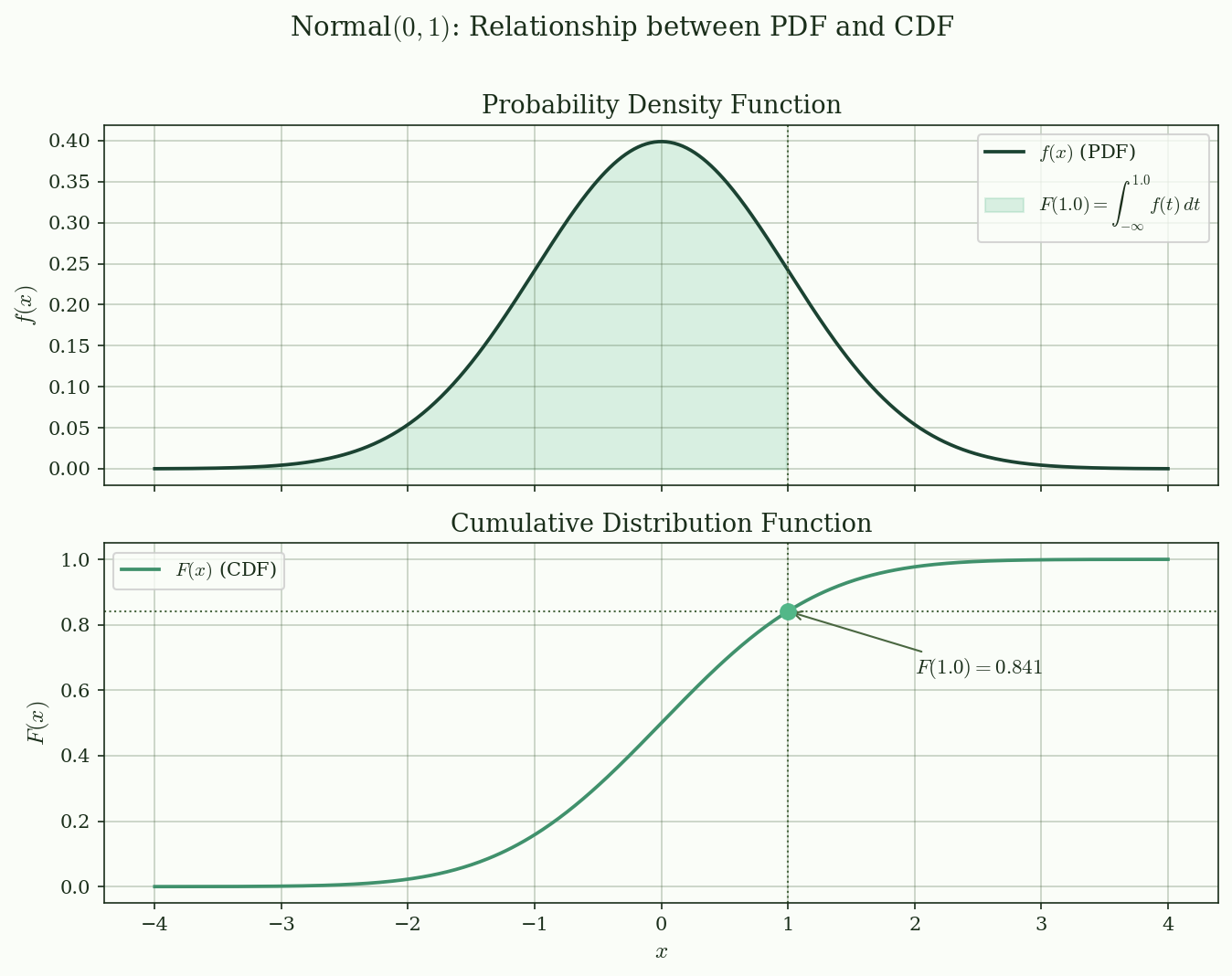{#fig-cdf}
## Transformations of Random Variables
Given a random variable $X$ with known distribution, suppose you define $Y = g(X)$. What is the distribution of $Y$?
### Discrete Case
If $X$ is discrete, collect all $x$ values that map to the same $y$:
$$
P(Y = y) = \sum_{\{x : g(x) = y\}} P(X = x)
$$
### Continuous Case (Change of Variables)
If $g$ is monotone and differentiable with inverse $g^{-1}$, the PDF of $Y$ is:
$$
f_Y(y) = f_X(g^{-1}(y)) \cdot \left| \frac{d}{dy} g^{-1}(y) \right|
$$
**Intuition first.** The factor $|dg^{-1}/dy|$ --- the **Jacobian** --- corrects for how the transformation stretches or compresses the number line. If $g$ squeezes a wide interval of $x$ into a narrow interval of $y$, the density must increase to keep the total probability at 1. The Jacobian measures exactly that stretching factor.
**Formally**, the absolute value of the derivative of the inverse function accounts for the change in "length" of infinitesimal intervals under the transformation.
### Example: $Y = X^2$, $X \sim N(0, 1)$
Since $g(x) = x^2$ is not monotone, split into $x > 0$ and $x < 0$ branches. The result is a $\chi^2(1)$ distribution:
$$
f_Y(y) = \frac{1}{\sqrt{2\pi y}} e^{-y/2}, \quad y > 0
$$
@fig-transformation shows the simulated histogram of $Y = X^2$ overlaid with the theoretical $\chi^2(1)$ density.
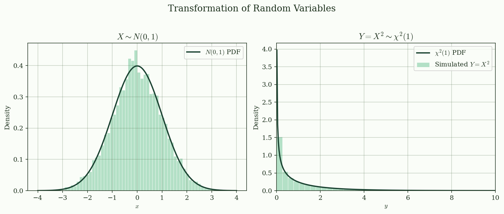{#fig-transformation}
## Practical Example: Simulation and Verification
How do you check whether a simulation matches a theoretical distribution? Two standard tools:
1. **Histogram overlay**: compare the empirical density to the theoretical PDF
2. **QQ plot**: plot sample quantiles against theoretical quantiles --- if the data follow the target distribution, the points lie on the 45-degree line
@fig-qq-plot shows a QQ plot for 100,000 samples drawn from $N(0, 1)$. The Kolmogorov--Smirnov test provides a formal check.
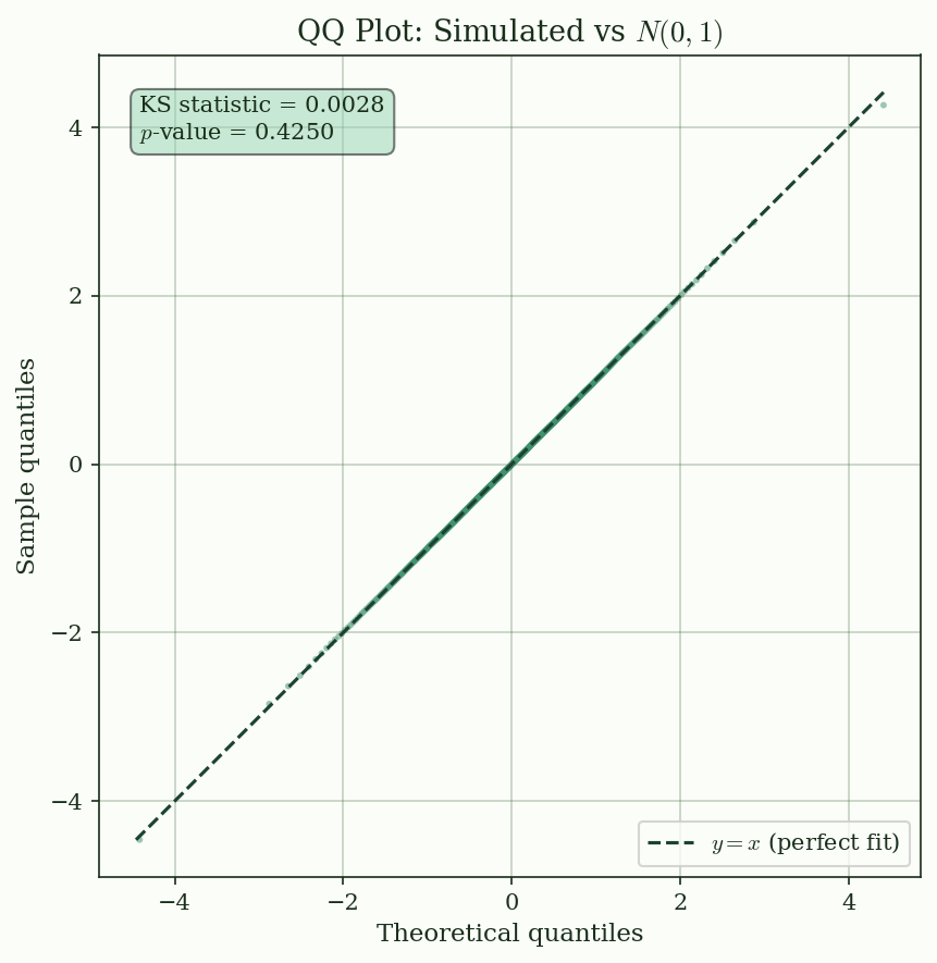{#fig-qq-plot}
## Summary and Connections
This article introduced random variables as the bridge from abstract probability spaces to numerical computation. The key takeaways:
- A random variable converts abstract outcomes into numbers you can compute with --- it is the reason we can use arithmetic in probability
- Discrete random variables have PMFs (bar charts); continuous ones have PDFs (curves where probability = area)
- The CDF unifies both cases and fully characterizes a distribution
- Transformations follow the change-of-variables formula, where the Jacobian corrects for stretching
- Simulation + QQ plots provide a practical way to verify distributional assumptions
**Next**: [Expectation and Variance](../expectation-variance/index.qmd) --- once you have a random variable, the natural next question is "what is its average value, and how spread out is it?"
**Application preview**: In credit risk modeling, a borrower's default is a Bernoulli random variable: $D \sim \text{Bernoulli}(PD)$, where $PD$ is the probability of default. The number of defaults in a portfolio is Binomial (under independence) or follows more complex distributions when correlation is present. The tools introduced here are the starting point for every risk model.
## References
::: {#refs}
:::


